5.1.5 Cumulative Frequency Graphs
In this topic we will learn how to:
- draw and interpret cumulative frequency graphs
A cumulative frequency graph is used to represent grouped continuous data. It is represented in the form of an s-shaped curve.
Cumulative frequency is the total frequency of the previous classes up to and including the present class.
To draw a cumulative frequency graph you need the following information:
- upper bound of a class
- cumulative frequency
To calculate the cumulative frequency, add the frequencies of previous classes together with that of the current class.\large\textcolor{gray}{\textbf{Variation and Measures of Central Tendency}\\ \textbf{ for Cumulative Frequency Graph}}\textbf{\textcolor{gray}{Mode}}A cumulative frequency curve represents grouped data, so we cannot find the mode but instead we can find the modal class. The modal class is the class with the highest frequency.\textcolor{gray}{n\textbf{-th percentile}}To calculate the n-th percentile, we use the formulan\textmd{-th percentile} = \frac{xn}{100}Where x represents the percentile and n represents the sample size.\textbf{\textcolor{gray}{Lower Quartile}}To calculate the lower quartile, we use the formula,
q_{1} = \frac{1}{4}nWhere q_{1} represents the lower quartile.\textbf{\textcolor{gray}{Upper Quartile}}To calculate the upper quartile, we use the formula,
q_{3} = \frac{3}{4}nWhere q_{3} represents the upper quartile.
\textbf{\textcolor{gray}{Intequartile Range}}To calculate the interquartile range, we use the formula,
IQR = q_{3} - q_{1}Where IQR represents the interquartile range, q_{3} represents the upper quartile, q_{1} represents the lower quartile.
\textbf{\textcolor{gray}{Mean}}To calculate the mean when data is displayed in the form of a cumulative frequency curve, we need to first find the mid interval. This is the middle value for each value. We use the formula,
\overline{x} = \frac{\Sigma xf}{\Sigma f}Where \overline{x} represents mean, x represents the mid-interval, f represents the frequency.
\textbf{\textcolor{gray}{Variance}}To calculate the variance, we use the formula,
\sigma^{2} = \frac{\Sigma x^{2}f}{\Sigma f} - \overline{x}^{2}Where \sigma^{2} represents variance, x represents the mid interval, f represents the frequency, \overline{x} represents mean.
\textbf{\textcolor{gray}{Standard Deviation}}Standard deviation is the square root of variance. Therefore, the formula for standard deviation is,
\sigma = \sqrt{\frac{\Sigma x^{2}f}{\Sigma f} - \overline{x}^{2}}Where \sigma represents standard deviation, x represents the mid interval, f represents the frequency, \overline{x} represents mean.
Let’s look at some past paper questions.
1. Helen measures the lengths of 150 fish of a certain species in a large pond. These lengths, correct to the nearest centimetre, are summarised, are summarised in the following table. (9709/52/F/M/20 number 7)
Length (cm) | 0 – 9 | 10 – 14 | 15 – 19 | 20 – 30 |
Frequency | 15 | 48 | 66 | 21 |
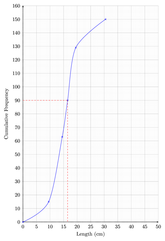
(a) Draw a cumulative frequency graph to illustrate the data.
Find the cumulative frequency,
Length (cm) | 0 – 9 | 10 – 14 | 15 – 19 | 20 – 30 |
Cumulative Frequency | 15 | 63 | 129 | 150 |
You will notice that there are gaps between the classes. To remove those gaps we need to do continuity correction. Simply subtract 0.5 from the lower bounds and add 0.5 to the upper bounds,
Length (cm) | 0 – 9.5 | 9.5 – 14.5 | 14.5 – 19.5 | 19.5 – 30.5 |
Cumulative Frequency | 15 | 63 | 129 | 150 |
Note: We do not subtract 0.5 from 0 because we would end up with a negative value for length, which does not exist.
Now that there are no gaps, we can plot the upper bounds against the cumulative frequency. Label the y-axis with cumulative frequency. Label the x-axis with the class title.

(b) 40\% of these fish have a length of d cm or more. Use your graph to estimate the value of d.
This means 60\% of fish have a length less than d cm. Let’s find 60\% of 150,
\frac{60}{100} \times 150\textcolor{red}{90}Draw construction lines at a cumulative frequency of 90 and read off the length,
d = 16.5 \textmd{ cm}Therefore, the final answer is,
d = 16.5 \textmd{ cm}The mean length of these 150 fish is 15.295 cm.
(c) Calculate an estimate for the variance of the lengths of the fish.
The formula for variance is,
\sigma^{2} = \frac{\Sigma x^{2}f}{\Sigma f} - \overline{x}^{2}We already have the mean, we need to find \frac{\Sigma x^{2}f}{\Sigma f}. x represents the mid intervals so let’s find x,
Mid Interval | 4.75 | 12 | 17 | 25 |
Frequency | 15 | 48 | 66 | 21 |
Note: Use the classes after continuity correction to find the mid interval.
Now that we have the mid interval, let’s find \frac{\Sigma x^{2}f}{\Sigma f},
\frac{\Sigma x^{2}f}{\Sigma f} = \frac{4.75^{2}(15) + 12^{2}(48) + 17^{2}(66) + 25^{2}(21)}{150}\frac{\Sigma x^{2}f}{\Sigma f} = 262.99653Note: Remember that f represents frequency NOT cumulative frequency.
Substitute into the formula for variance,
\sigma^{2} = \frac{\Sigma x^{2}f}{\Sigma f} - \overline{x}^{2}\sigma^{2} = 262.99653 - (15.295)^{2}\sigma^{2} = 29.059225\sigma^{2} = 29.1Therefore, the final answer is,
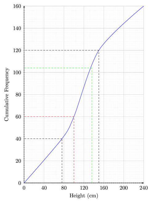
\sigma^{2} = 29.12. The heights in cm of 160 sunflower plants were measured. The results are summarised on the following cumulative frequency curve. (9709/53/M/J/21 number 1)

(a) Use the graph to estimate the number of plants with heights less than 100 cm.
Draw construction lines at the height of 100 cm and read off the respective cumulative frequency,
\textcolor{red}{60}Therefore, the final answer is,
60 \textmd{ plants}(b) Use the graph to estimate the 65th percentile of the distribution.
The formula to find the nth percentile is,
\frac{xn}{100}Substitute the value of x and n,
\frac{(65)(160)}{100}104Draw construction lines at a cumulative frequency of 104 and read off the respective height,
\textcolor{#0f0}{136}Therefore, the final answer is,
136(c) Use the graph to estimate the interquartile range of the heights of these plants.
The formula to find the interquartile range is,
IQR = q_{3} - q_{1}To find the upper quartile, use the formula,
q_{3} = \frac{3}{4}nq_{3} = \frac{3}{4}(160)q_{3} = 120Draw construction lines at a cumulative frequency of 120 and read off the respective height,
q_{3} = 150To find the lower quartile, use the formula,
q_{1} = \frac{1}{4}nq_{1} = \frac{1}{4}(160)q_{1} = 40Draw construction lines at a cumulative frequency of 40 and read off the respective height,
q_{1} = 76Substitute into the formula for interquartile range,
IQR = q_{3} - q_{1}IQR = 150 - 76IQR = 74Therefore, the final answer is,
IQR = 74
